Introduction

BasisPoint recently contributed an implementation of zero coupon swaps in the open source financial library QuantLib.

This short article presents how to value and calculate basic risk characteristics of a zero coupon swap. Also, a brief summary of the methodology is given to better understand the implementation.

The presented examples are freely available in a GitHub repository, and can be run and tested online.

What can zero coupon swaps be used for?

Zero coupon swap is a derivative which exchanges only two single cash flows at maturity. One of its legs assumes a fixed cash flow payment, whereas the other is linked to a floating rate which is periodically compounded.

These derivatives can be of particular use for pension funds as a hedging instrument for their long-dated liabilities. Given that the cash flows are exchanged at maturity only, it is easier to perform cash flow matching operations compared to e.g. vanilla interest rate swaps. A considerable downside, which also stems from the cash flows being paid only at maturity, is significantly higher counterparty risk as opposed to vanilla IRSes (that pay coupons). This leads to somewhat smaller popularity of these derivatives among other market participants – in consequence lower liquidity and relatively higher pricing levels.

Valuation

Zero coupon swaps can be quoted in terms of a known fixed cash flow N^FIX or a fixed rate R, where:

N^FIX = N [(1 + R)^{α(T₀, T_K)} − 1]

with α(T₀, T_K) being the time fraction between the start date of the contract T₀ and the end date T_K – according to a given day count convention. N is the base notional amount prior to compounding.

The floating leg also pays a single cash flow N^FLT, which value is determined by periodically averaging (e.g. every 6 months) interest rate index fixings.

Assuming the use of compounded averaging the projected value of the floating leg becomes:

N^FLT = N [∏_k=0^K−1 (1 + α(T_k, T_k+1) L(T_k, T_k+1)) − 1]

where L(T_i, T_j) are interest rate index fixings for accrual period [T_i, T_j].

The present value of a receiver contract (one in which the fixed leg cash flow is received) is:

V(t) = P(t, T) N^FIX − P(t, T) N^FLT

where T is the final payment time (T > T_K), P(t, T) is the nominal discount factor at time T with reference time t.

Given that the payoff on the floating leg of a zero coupon swap is compounded, it is of great importance for valuation and risk management to be able to project relatively reliable future Euribor fixings. The quality of the forwards largely depends on the chosen interpolation scheme for the term structure (next to reliable market data). We will demonstrate a number of examples of forward curves given different interpolation schemes.

Based on the shapes of the presented term structures, a number of conclusions can be drawn:

• linear interpolation on zero rates exhibits a saw-tooth shaped forward curve, which suggests poor stability of the index projections;
• cubic interpolation on zero rates shows some improvement, compared to linear interpolation, still the forwards are showing fluctuations which are not desired;
• linear interpolation on log discounts leads to a staircase shaped forward curve, which means that between the nodes of the curve, forwards are kept constant;
• cubic interpolation on log discounts produces a smooth forward curve, which also seems closest to the economic expectations.

Assume, we want to value a 25 years receiver swap, which started a few years ago and has still around 20 years to maturity, with EUR 10 million as base notional and a fixed rate of 1%. We will observe the following valuations depending on the interpolation scheme:

• NPV using linear zero interpolation: EUR 1,795,966
• NPV using linear log discount interpolation: EUR 1,794,153
• NPV using cubic zero interpolation: EUR 1,788,657
• NPV using cubic log discount interpolation: EUR 1,778,770.

Risk analysis

The library offers a number of methods to analyse the risks associated with this instrument.

We are going to focus here on the par deltas, being the sensitivity of the market value of the instrument with respect to changes of the par swap rates constituing the term structure used to discount the cash flows and to project the future interest rate fixings of the instrument.

In the end we obtain some interesting sensitivity distributions for various interpolation methods.

The graphs below demonstrate the distributions of the par deltas depending on the interpolation scheme.

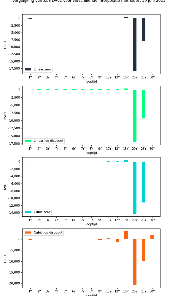
The sensitivities calculated under a term structure using cubic zero and cubic log discount interpolations are visibly different, compared to the profile under the remaining two schemes. In fact, it is very often the case that cubic interpolation schemes display an issue of non-locality of hedges.

The aggregated DV01s are:

• DV01 using linear zero interpolation: EUR -25,795
• DV01 using linear log discount interpolation: EUR -24,665
• DV01 using cubic zero interpolation: EUR -25,767
• DV01 using cubic log discount interpolation: EUR -25,799.

Total DV01s are close to each other, but it is the distribution of deltas that portfolio managers or traders might look at when sizing hedges.

It is also worthwhile to note that the valuation differences resulting from different interpolation schemes are within one DV01, which is associated with a parallel shift of the valuation curve by one basis point. That is also typically considered as an acceptable threshold for valuation difference for this type of derivatives.

For questions and remarks, regarding this blog post, any other blog post or the services that BasisPoint can provide, please feel free to contact us via info@basispoint.io.